Get started with ccsgp!

Authors

Patrick Huck (GitHub), default_colors in pyana.ccsgp.config contributed by Johanna Huck

Date

July 29, 2014

If the documentation here doesn’t contain screenshots it didn’t build correctly. In that case, please find a static manually uploaded version at http://downloads.the-huck.com/ccsgp_get_started/

This package provides a sample setup to get started with ccsgp. ccsgp is initialized as a module and its usage demonstrated with dedicated functions in the examples module. Helpful utility functions are also included to complement the features of ccsgp. The following use cases are currently implemented or will be in the future:

• keep input/output directory layouts according to the module’s structure
• load data from text files with the correct column formats
• import data from ROOT objects via root-py
• and more ...

Please submit tickets on GitHub issues.

Installation

1. ccsgp_get_started requires gnuplot, git, virtualenv and optionally hdf5. Install these dependencies via:

   $ sudo port install gnuplot git-core py27-virtualenv [hdf5] # MacPorts
   $ sudo apt-get install gnuplot git python-virtualenv [libhdf5-dev] # Debian/Ubuntu
   

   hdf5 is optional but if you’d like to save your image data to HDF5, you’ll have to install it.

2. clone the ccsgp_get_started git repository:

   $ git clone https://github.com/tschaume/ccsgp_get_started.git --recursive
   $ cd ccsgp_get_started/
   

3. init the virtualenv, activate it and install all requirements:

   $ virtualenv-2.7 env
   $ source env/bin/activate
   $ pip install -U numpy
   $ pip install -U -r requirements.txt --allow-external gnuplot-py --allow-unverified gnuplot-py
   

   Every time you start in a new terminal you have to activate the correct python environment by sourcing env/bin/activate again or instead use env/bin/python directly!

   The h5py package is currently omitted from the requirements. If you want to use it, uncomment the h5py requirement in requirements.txt and rerun $ pip install -r requirements.txt.

4. If you intend to run the examples, clone the test data repository (somewhere outside of ccsgp_get_started repository):

   $ git clone http://gitlab.the-huck.com/github/ccsgp_get_started_data.git
   

   and symlink pyanaDir to the ccsgp_get_started_data directory:

   $ cd ccsgp_get_started/
   $ ln -s <path/to/ccsgp_get_started_data> pyanaDir
   

   pyana.aux.utils.checkSymLink checks for the pyanaDir symbolic link and the code won’t run without it. Hence you need to generate a symlink called pyanaDir either to ccsgp_get_started_data or your own input/output directory (preferably separated from the code repository).

   Pull in public STAR dielectron data into a new branch to use gp_xfac and gp_panel:

   $ cd <path/to/ccsgp_get_started_data>
   $ git remote add dielec_public http://gitlab.the-huck.com/star/dielectron_data_public.git
   $ git checkout -b star_dielec
   $ git pull dielec_public master
   

   If you are part of the STAR collaboration you can also pull in the protected STAR dielectron data to include it in gp_panel:

   $ git remote add dielec_protect http://cgit.the-huck.com/dielectron_data_protected
   $ git pull -Xtheirs dielec_protect master
     (enter STAR protected credentials)
   

Examples Module

The examples are based on a dataset of World Bank Indicators. You can use the dataset yourself to play around [1]. See the genExDat.sh script in the same directory on how I extracted the data into the correct format for ccsgp. To generate all example plots based on ccsgp_get_started_data you can run:

$ python -m pyana

[1]	ccsgp_get_started_data/input/examples/gp_datdir/{WorldBankIndicators.csv, genExDat.sh}

Alternatively, you can run a specific module, for instance:

$ python -m pyana.examples.gp_datdir [--log] <country-initial> <#-most-populated>

and this way plot specific country initials. You can open all resulting pictures via $ open examplesDir/examples/gp_datdir/*.pdf or use pdfnup to put multiple plots on one page. To start on your own read the documentation below or the source code and use one of the examples as a template.

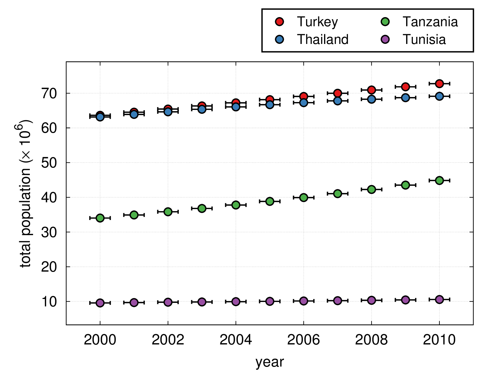
pyana.examples.gp_datdir.gp_datdir(initial, topN)

example for plotting from a text file via numpy.loadtxt

1. prepare input/output directories
2. load the data into an OrderedDict() [adjust axes units]
3. sort countries from highest to lowest population
4. select the <topN> most populated countries
5. call ccsgp.make_plot with data from 4

Below is an output image for country initial T and the 4 most populated countries for this initial (click to enlarge). Also see:

$ python -m pyana.examples.gp_datdir -h

for help on the command line options.

Parameters:

• initial (str) – country initial
• topN (int) – number of most populated countries to plot

Variables:

• inDir – input directory according to package structure and initial
• outDir – output directory according to package structure
• data – OrderedDict with datasets to plot as separate keys
• file – data input file for specific country, format: [x y] OR [x y dx dy]
• country – country, filename stem of input file
• file_url – absolute url to input file
• nSets – number of datasets

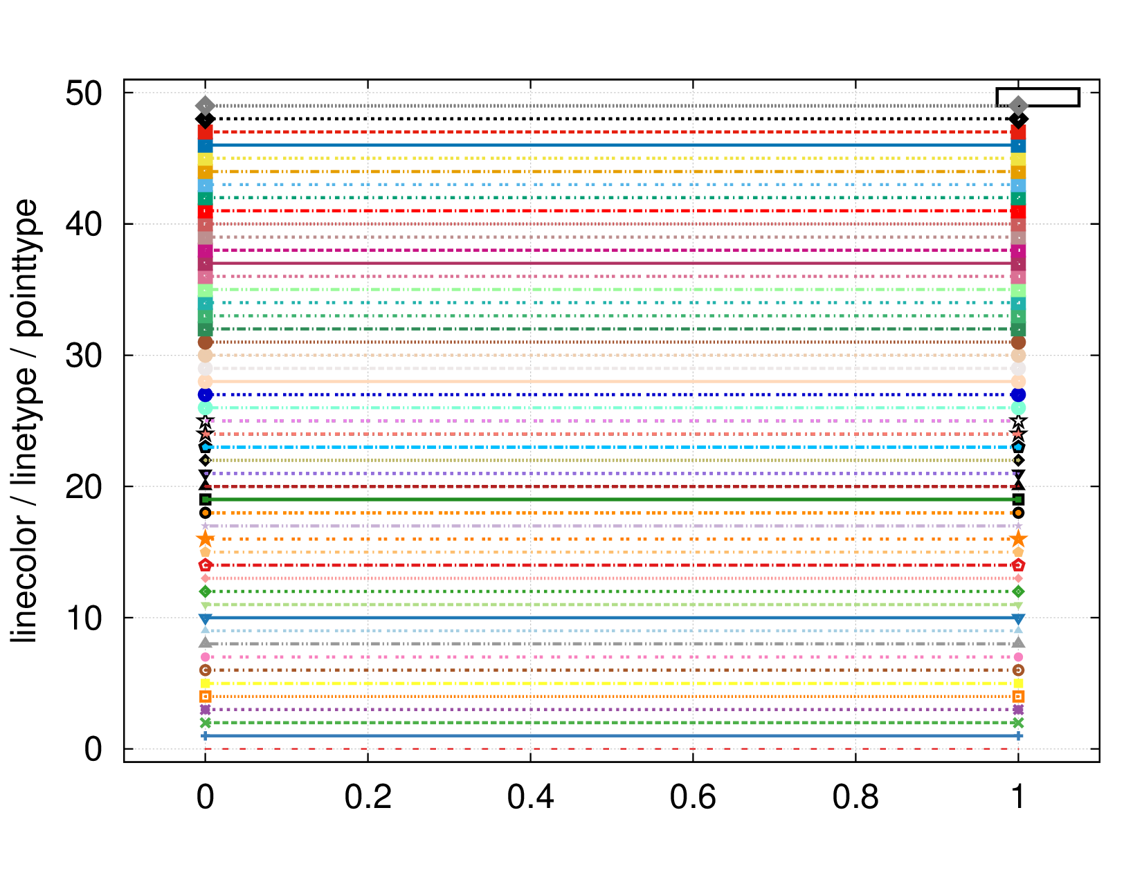
pyana.examples.gp_lcltpt.gp_lcltpt()

example plot to display linecolors, linetypes and pointtypes

pyana.examples.gp_xfac.gp_xfac()

example using QM12 enhancement factors

• uses gpcalls kwarg to reset xtics
• numpy.loadtxt needs reshaping for input files w/ only one datapoint
• according poster presentations see QM12 & NSD review

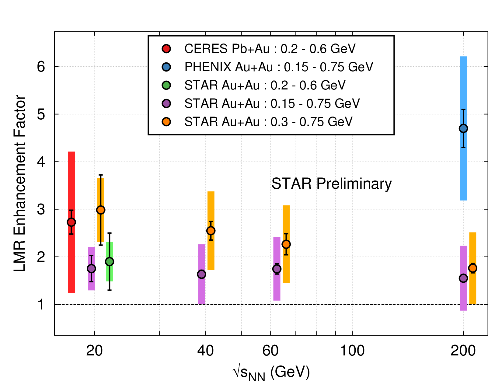
Variables:

• key – translates filename into legend/key label
• shift – slightly shift selected data points

pyana.examples.gp_panel.gp_panel(version, skip)

example for a panel plot using QM12 data (see gp_xfac)

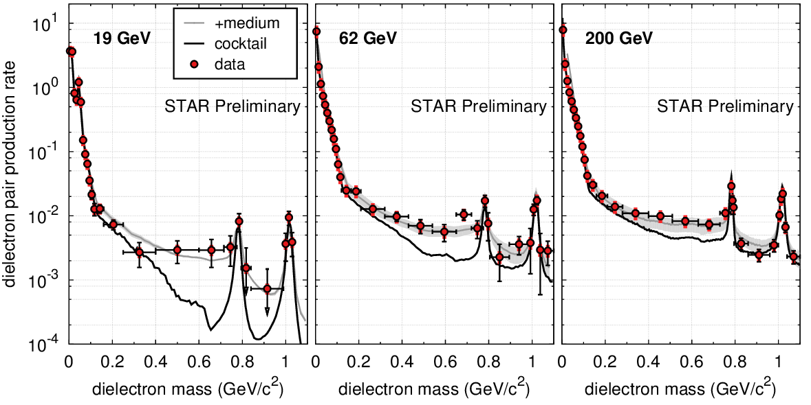
Parameters:version (str) – plot version / input subdir name

pyana.examples.gp_stack.gp_stack(version, energies, inclMed, inclFits)

example for a plot w/ stacked graphs using QM12 data (see gp_panel)

• how to omit keys from the legend
• manually add legend entries
• automatically plot arrows for error bars larger than data point value

Parameters:version (str) – plot version / input subdir name

pyana.examples.gp_rdiff.gp_rdiff(version, nomed, noxerr, diffRel, divdNdy)

example for ratio or difference plots using QM12 data (see gp_panel)

• uses uncertainties package for easier error propagation and rebinning
• stat. error for medium = 0!
• stat. error for cocktail ~ 0!
• statistical error bar on data stays the same for diff
• TODO: implement ratio!
• TODO: adjust statistical error on data for ratio!
• TODO: adjust name and ylabel for ratio

Parameters:

• version (str) – plot version
• nomed (bool) – don’t plot medium
• noxerr (bool) – don’t plot x-errors

pyana.examples.gp_ptspec.gp_ptspec()

example for a 2D-panel plot etc.

pyana.examples.utils.checkSymLink()

check for symbolic link to input directory

pyana.examples.utils.enumzipEdges(eArr)

zip and enumerate edges into pairs of lower and upper limits

pyana.examples.utils.getCocktailSum(e0, e1, eCocktail, uCocktail)

get the cocktail sum for a given data bin range

pyana.examples.utils.getEdges(npArr)

get np array of bin edges

pyana.examples.utils.getMaskIndices(mask)

get lower and upper index of mask

pyana.examples.utils.getUArray(npArr)

uncertainty array multiplied by binwidth (col2 = dx)

pyana.examples.utils.getWorkDirs()

get input/output dirs (same input/output layout as for package)

ccsgp

ccsgp is a plotting library based on gnuplot-py which wraps the necessary calls to gnuplot-py into one function called make_plot. The keyword arguments to make_plot provide easy control over the plot-by-plot dependent options while reasonable defaults for legend, grid, borders, font sizes, terminal etc. are handled internally. By providing the data in a default and reasonable format, the user does not need to deal with the details of “gnuplot’ing” nor the internals of the gnuplot-py interface library. Every call of make_plot dumps an ascii representation of the plot in the terminal and generates the eps hardcopy original. The eps figure is also converted automatically into pdf, png and jpg formats for easy inclusion in presentations and papers. In addition, the user can decide to save the data contained in each image into hdf5 files for easy access via numpy. The function repeat_plot allows the user replot a specific graph with different properties, like axis ranges for instance. The make_panel user function facilitates plotting of 1D- or 2D-panel images with merged axes.

The name ccsgp stands for “Carbon Capture and Sequestration GnuPlot” as this library started off in the context of my wife’s research. I knew how to produce nice-looking plots using gnuplot but wanted to hook it up to python directly. The resulting library let’s me generate identical plots independent of the data input source (ROOT, YAML, txt, pickle, hdf5, ...) using the full power of python.

User Functions

pyana.ccsgp.ccsgp.make_panel(dpt_dict, **kwargs)

make a panel plot

• name/title/debug are global options used once to initialize the multiplot
• x,yr/x,ylog/lines/labels/gpcalls are applied on each subplot
• key/ylabel are only plotted in first subplot
• xlabel is centered over entire panel
• same for r,l,b,tmargin where r,lmargin will be reset, however, to allow for merged y-axes
• input: OrderedDict w/ subplot titles as keys and lists of make_plot’s data/properties/titles as values, see below
• layout = ‘<cols>x<rows>’, defaults to horizontal panel if omitted

Parameters:dpt_dict (dict) – OrderedDict('subplot-title': [data, properties, titles], ...)

pyana.ccsgp.ccsgp.make_plot(data, properties, titles, **kwargs)

main function to generate a 1D plot

• each dataset is represented by a numpy array consisting of data points in the format [x, y, dx, dy1, dy2], dy1 = statistical error, dy2 = systematic uncertainty
• for symbol numbers to use in labels see http://bit.ly/1erBgIk
• lines format: ‘<x/y>=<value>’: ‘<gnuplot options>’, horizontal = (along) x, vertical = (along) y
• labels format: ‘label text’: [x, y, abs. placement true/false]
• arrows format: [<x0>, <y0>], [<x1>, <y1>], ‘<gnuplot props>’

Parameters:

• data (list) – datasets
• properties (list) – gnuplot property strings for each dataset (lc, lw, pt ...)
• titles (list) – legend/key titles for each dataset
• name (str) – basename of output files
• title (str) – image title
• debug (bool) – flag to switch to debug/verbose mode
• key (list) – legend/key options to be applied on top of default_key
• xlabel (str) – label for x-axis
• ylabel (str) – label for y-axis
• xr (list) – x-axis range
• yr (list) – y-axis range
• xlog (bool) – make x-axis logarithmic
• ylog (bool) – make y-axis logarithmic
• lines (dict) – vertical and horizontal lines
• arrows (list) – arrows
• labels (dict) – labels
• lmargin (float) – defines left margin size (relative to screen)
• bmargin (float) – defines bottom margin size
• rmargin (float) – defines right margin size
• tmargin (float) – defines top margin size
• arrow_offset (float) – offset from data point for special error bars (see gp_panel)
• arrow_length (float) – length of arrow from data point towards zero for special error bars (see gp_panel)
• arrow_bar (float) – width of vertical bar at end of special error bars (see gp_panel)
• gpcalls (list) – execute arbitrary gnuplot set commands

Returns:

MyPlot

pyana.ccsgp.ccsgp.repeat_plot(plt, name, **kwargs)

repeat a plot with different properties (kwargs see make_plot)

Parameters:

• plt (MyPlot) – plot to repeat
• name (str) – basename of new output file(s)

Returns:

plt

Base Class

class pyana.ccsgp.myplot.MyPlot(name='test', title='', debug=0)

base class

• basic gnuplot setup (bars, grid, title, key, terminal, multiplot)
• utility functions for general plotting

Parameters:

• title (str) – image title
• name (str) – basename used for output files
• debug (bool) – debug flag for verbose gnuplot output

Variables:

• name – basename for output files
• epsname – basename + ‘.eps’
• gp – Gnuplot.Gnuplot instance
• nPanels – number of panels in a multiplot
• nVertLines – number of vertical lines
• nLabels – number of labels
• nArrows – number of arrows
• axisLog – flags for logarithmic axes
• axisRange – axis range for respective axis (set in setAxisRange)

_ascii()

write ascii file(s) w/ data contained in plot

_clamp(val, minimum=0, maximum=255)

convenience function to clamp number into min..max range

_colorscale(hexstr, scalefactor=1.4)

Scales a hex string by scalefactor. Returns scaled hex string.

• taken from T. Burgess (source)
• To darken the color, use a float value between 0 and 1.
• To brighten the color, use a float value greater than 1.

>>> colorscale("#DF3C3C", .5)
#6F1E1E
>>> colorscale("#52D24F", 1.6)
#83FF7E
>>> colorscale("#4F75D2", 1)
#4F75D2

_convert()

convert eps/ps original into pdf, png and jpg format

_get_style_mod_prop(prop)

get style and modified property string

_hardcopy()

generate eps, convert to other formats and write data to hdf5

_hdf5()

write data contained in plot to HDF5 file

• easy numpy import -> (savetxt) -> gnuplot
• export to ROOT objects

h5py howto (see http://www.h5py.org/docs/intro/quick.html):

• open file: f = h5py.File(name, ‘r’)
• list datasets: list(f)
• load entire dataset as np array: arr = f[‘dset_name’][...]
• NOTE: literally type the 3 dots, replace dset_name
• np.savetxt format: fmt = ‘%.4f %.3e %.3e %.3e %.3e’
• save array to txt file: np.savetxt(‘arr.dat’, arr, fmt=fmt)

Raises:ImportError

_plot_errs(data)

determine whether to plot primary errors separately

plot errorbars if data has more than two columns which are not all zero

Parameters:data (numpy.array) – one dataset Variables:error_sums – sum of x and y errors Returns:True or False

_plot_syserrs(data)

determine whether to plot secondary errors

Parameters:data (numpy.array) – one dataset Returns:True or False

_prettify(str)

prettify string, remove special symbols

_setter(list)

convenience function to set a list of gnuplot options

Parameters:list (list) – list of strings given to gnuplot’s set command

_sum_errs(data, i)

convenience function to calculate sum of i-th column

_using(data, prop=None)

determine string with columns to use

Parameters:

• data (numpy.array) – one dataset
• prop (str) – property string of a dataset

Returns:

‘1:2:3’, ‘1:2:4’ or ‘1:2:3:4’

_with_errs(data, prop)

generate special property string for primary errors

• currently error bars are drawn in black
• use same linewidth as for points
• TODO: give user the option to draw error bars in lighter color according to the respective data points

Parameters:

• data (numpy.array) – one dataset
• prop (str) – property string of a dataset

Returns:

property string for primary errors

_with_main(prop)

get the correct property string for main data

_with_syserrs(prop)

generate special property string for secondary errors

• draw box in lighter color than point/line color
• does not support integer line colors, only hex

Parameters:prop (str) – property string of a dataset Returns:property string for secondary errors

addHorizontalLine(y, opts)

draw horizontal line

Parameters:

• y (float) – y-position
• opts (str) – line draw options

getMargin(margin, **kwargs)

get global margins

initData(data, properties, titles, subplot_title=None)

initialize the data

• all lists given as parameters must have the same length.
• each data set is drawn twice to allow for different colors for the errorbars
• error bars use the same linewidth as data points and line color black
• use ‘boxwidth 0.03 absolute’ in gp_calls to set the width of the uncertainty boxes
• use alternative gnuplot style if properties contains a style specification in the form with <style> and if the style is in ccsgp.config.supported_styles (style specification has to be at the beginning of the property string!)

Parameters:

• data (list of numpy arrays) – data points w/ format [x, y, dx, dy] for each dataset
• properties (list of str) – plot properties for each dataset (pt/lw/ps/lc...)
• titles (list of strings) – key/legend titles for each dataset
• subplot_title (str) – subplot title for panel plot case

Variables:

• dataSets – zipped titles and data for hdf5/ascii output and setAxisRange
• data – list of Gnuplot.Data including extra data sets for error plotting

plot(hardcopy=True)

plot and generate output files

prepare_plot(**kwargs)

prepare for plotting (calls all members of MyPlot)

setArrow(p0, p1, prop)

draw an arrow into the figure

Parameters:

• p0 (list) – start point [x, y]
• p1 (list) – end point [x, y]
• prop (str) – gnuplot property string for the arrow

setAxisLabel(label, axis='x')

set label for specified axis

Parameters:

• label (str) – label
• axis (str) – axis which to label

setAxisLog(log, axis='x')

set logarithmic scale for specified axis

Parameters:

• log (bool) – whether to set logarithmic
• axis (str) – axis which to set logarithmic

setAxisLogs(**kwargs)

set axes logarithmic if requested

setAxisRange(rng, axis='x')

set range for specified axis

• automatically determines axis range to include all data points if range is not given.
• logscale and secondary errors taken into account
• y-axis range determined for points within given x-axis range

Parameters:

• rng (list) – lower and upper range limits
• axis (str) – axis to which to apply range

setErrorArrows(**kwargs)

reset properties of arrows used to plot special errors

setKeyOptions(key_opts)

set key options

Parameters:key_opts (list) – strings for key/legend options

setLabel(label, pos, abs_place=False)

draw a label into the figure

Parameters:

• label (str) – label
• pos (list) – x,y - position
• abs_place (bool) – absolute or relative placement

setMargins(**kwargs)

set the margins

• keys other than l(b,t,r)margin are ignored (see config.default_margins)

setVerticalLine(x, opts)

draw a vertical line

Parameters:

• x (float) – position on x-axis
• opts (str) – line draw options

Config & Utils

var default_key:  default options for legend/key var basic_setup:  bars, grid, terminal and default_key var default_margins:  default margins to define plot area var xPanProps:xscale, xsize, xoffset for panel plots var default_colors:  provides a reasonable color selection (see palette)

pyana.ccsgp.utils.getOpts(i)

convience function for easy access to gnuplot property string

pyana.ccsgp.utils.zip_flat(a, b, c=None)

zips two or three lists and flattens the result

Indices and tables

• Index
• Module Index
• Search Page